SiO2/HfO2 (001) Valence Band Offset
1. Introduction
This tutorial calculates the valence band offset ΔE_v of two SiO₂/HfO₂ (001) superlattices, one with monoclinic and one with cubic HfO₂, reproducing the results of the following manuscripts:
Manuscripts
Pierre-Yves Prodhomme, Fabien Fontaine-Vive, Abram Van Der Geest, Philippe Blaise and Jacky Even, "Ab initio calculation of effective work functions for a TiN/HfO2/SiO2/Si transistor stack", Applied Physics Letters 99, 022101 (2011). DOI: 10.1063/1.3609869. 1
John Robertson and Robert M. Wallace, "High-K materials and metal gates for CMOS applications", Materials Science and Engineering: R: Reports 88, 1 (2015). DOI: 10.1016/j.mser.2014.11.001. 2
This tutorial builds upon the SiO2/HfO2 (001) Superlattices with Monoclinic and Cubic HfO2 tutorial, where the two superlattices and their three bulk cells are created. Here, the notebook anneals the monoclinic superlattice and relaxes both with the MACE-MP-0 machine-learned force field, and the platform's Valence Band Offset (Bulk Method) workflow runs Quantum ESPRESSO on each relaxed superlattice and its two bulk cells. The offset is assembled by the potential lineup 3: each bulk's valence band maximum E_VBM is measured from its own average potential V̄, and the superlattice gives the step in V̄ between the two materials,
1 | |
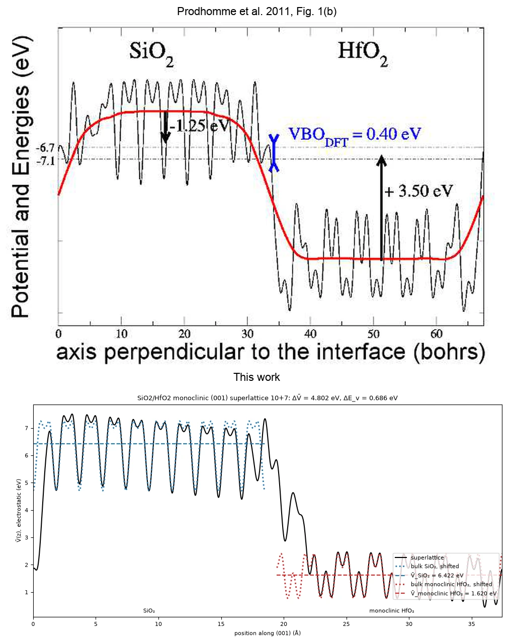
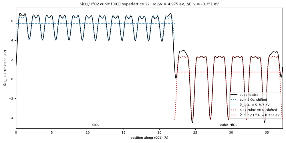
ΔE_v is positive when the valence band maximum of SiO₂ lies above that of HfO₂, the sign convention of both manuscripts. In the local density approximation (LDA), Prodhomme et al. give ΔE_v = +0.4 eV for the monoclinic model (Table I), and Robertson and Wallace −0.67 eV for the cubic model (Fig. 57a).
2. Prerequisites
Before starting this tutorial, one of the following steps should be completed:
- Follow the SiO2/HfO2 (001) Superlattices tutorial, using
the
interface_3d_3d_silicon_dioxide_hafnium_dioxide.ipynbnotebook embedded in its section 6, to create and saveSiO2/HfO2 monoclinic (001) superlattice 10+7,SiO2/HfO2 cubic (001) superlattice 12+6,SiO2 beta-cristobalite (001) bulk,HfO2 monoclinic (001) bulk strainedandHfO2 cubic (001) bulk strained, OR - Have the five materials saved in the
uploadsfolder or in the account's materials collection
3. Workflow overview
The calculation consists of the following steps:
- Set up the environment and parameters: Configure the material names, the Density Functional Theory (DFT) model, the anneal and relaxation, and compute resources
- Authenticate and initialize API client: Connect to the platform
- Load materials: Import the two superlattices and the three bulks, print their composition and geometry
- Configure the model and k-grids: One DFT model, the same k-grid for both superlattices, a k-grid per bulk from one k-point density
- Configure compute resources: Select the cluster, queue, and processor settings
- Anneal the monoclinic superlattice: Molecular dynamics on the MACE-MP-0 force field, from 1000 K to 100 K in 1 ps, as Prodhomme et al.
- Relax the superlattices: Atomic positions at fixed cell on the same force field, to 0.07 eV/Å
- Configure the workflow: One Valence Band Offset (Bulk Method) workflow per superlattice, with the model and a k-grid per material
- Run the jobs: One job per superlattice, which runs the electrostatic potential of the superlattice, the band structure and the electrostatic potential of each bulk, and the offset
- Retrieve results: The offsets and the potential profiles, and the potential across each superlattice
- Compare with the manuscripts: Print each offset beside its manuscript's value
4. Calculation parameters
| this tutorial | Prodhomme et al. | Robertson and Wallace | |
|---|---|---|---|
| HfO₂ phase | monoclinic and cubic | monoclinic (P2₁/c) | cubic, after Sharia et al. 4 |
| Code | Quantum ESPRESSO | SIESTA | not given in the review |
| Functional | LDA: Ceperley–Alder, Perdew–Zunger parametrization | LDA: Ceperley–Alder | LDA |
| Basis and pseudopotentials | plane waves, ultrasoft, Garrity–Bennett–Rabe–Vanderbilt (GBRV) LDA library | double-zeta polarized atomic orbitals, Troullier–Martins norm-conserving | not given in the review |
| Cutoff | 40 / 200 Ry | mesh cutoff of at least 100 Ha | not given in the review |
| k-points | 4×4×1 for both superlattices, as Sharia et al.; 3.5 points per Å⁻¹ for the bulks: 5×5×3 SiO₂, 5×5×5 HfO₂ | not given | not given in the review; Sharia et al.: 4×4×1 for the interface, 8×8×8 for the bulks |
| Cell | monoclinic: 10 + 7 layers, Hf₁₄Si₁₀O₄₈; cubic: 12 + 6 layers, Hf₁₂Si₁₂O₄₈; 72 atoms each, 5.2317 × 5.2317 Ų | seven HfO₂ layers, ten SiO₂ tetrahedra, 5.23 × 5.23 Ų | 4 O per HfO₂ layer, 2 per SiO₂ layer, 3 in the interface plane |
| Lattice | the Standata structures, HfO₂ strained in plane onto SiO₂ | LDA lattices, HfO₂ stretched by 3.7 % along [100] and 2.1 % along [010] | not given in the review |
| Positions | MACE-MP-0, trained on Perdew–Burke–Ernzerhof (PBE) data, fixed cell: monoclinic annealed from 1000 K to 100 K in 1 ps, then both relaxed to 0.07 eV/Å; the cation layer on each side of an interface and the atoms between them move, the block interiors stay at the bulk crystals | LDA: anneal from 1000 K to 100 K in 1 ps, then conjugate gradient to 0.07 eV/Å | LDA, relaxed |
| Offset | potential lineup: V̄ of each bulk the mean of its planar-averaged electrostatic potential; V̄ in the superlattice at each block's centre, from the planar average smoothed by a double convolution with the two bulks' (001) layer spacings | potential lineup, planar average smoothed by a double convolution | local densities of states of HfO₂ and SiO₂ layers away from the interface |
| Band-edge corrections | not computed | G0W0 corrections to the bulk band edges, listed separately in Table I | not given in the review |
5. Step-by-step instructions
5.1. Open the notebook
Navigate to the API examples repository and open the notebook:
1 | |
5.2. Configure parameters
Cells 1.2-1.5 set the material names, the compute resources, the DFT model, and the anneal and relaxation:
1 2 3 4 5 6 7 8 9 10 11 12 13 14 15 16 17 18 19 20 21 22 23 24 25 26 27 28 29 30 31 32 33 34 35 36 37 38 39 40 41 42 43 44 45 46 47 48 49 50 51 52 | |
5.3. Run the notebook
Execute all cells by selecting Run > Run All from the menu.
The notebook first authenticates with the platform, then runs the steps listed in section 3.
5.4. Analyze results
Section 3 of the notebook prints the composition and the cell of the five materials, and the (001) layer spacing of each bulk:
1 2 3 4 5 6 7 8 | |
The (001) layer spacings are the widths of the double convolution in the superlattice, one period of the potential in each block. Section 10.1 reads the offset of each superlattice from the valence band offset property its job stores, and section 10.2 plots the potential across both superlattices with the bulk potentials overlaid.
The last cell prints, for each model, the manuscript's value and then the value of this calculation:
1 2 | |
6. Expected results
Table I of Prodhomme et al. lists the valence band offset (VBO) VBO(LDA) = +0.4 eV for SiO₂/HfO₂, the valence band of SiO₂ above that of HfO₂; their Fig. 1(b) marks it as 0.40 eV. The same table lists −1.0 eV after their G0W0 corrections, which are not computed here. Fig. 57a of Robertson and Wallace gives −0.67 eV for the undoped interface, the "Hf" point, read off the figure: the valence band of HfO₂ above that of SiO₂.
6.1. Comparison with published results
| Model | Manuscript | ΔE_v, manuscript (eV) | ΔE_v, this tutorial (eV) |
|---|---|---|---|
| monoclinic HfO₂ | Prodhomme et al., Table I | +0.4 | +0.69 |
| cubic HfO₂ | Robertson and Wallace, Fig. 57a | −0.67 | −0.35 |
Fig. 1(b) of Prodhomme et al. shows the potential across their monoclinic superlattice, SiO₂ on the left (black), and its double-convolution average (red); the arrows mark each bulk's valence band maximum against its averaged potential and the offset. Section 10.2 of the notebook draws the monoclinic superlattice of this tutorial in the same orientation, below it: one period from the HfO₂→SiO₂ interface, the planar average (black), each bulk's own potential (dotted) shifted onto its block, and the two block averages over one (001) layer (dashed):
The cubic superlattice, drawn the same way:
7. Customization options
7.1. Adjust computational resources
CLUSTER_NAME selects the cluster by its full or partial name; a name that is not available makes the notebook
stop and list the ones that are. Without a name, the first cluster of the account is used.
8. Troubleshooting
8.1. Material not found
If one of the five names is not found, run the
SiO2/HfO2 (001) Superlattices tutorial first. In JupyterLite,
save the five materials to the account from Materials Designer under those exact names; in a local Jupyter session,
check that the uploads folder holds them.
8.2. No cluster available
If section 5.1 of the notebook prints an empty list of clusters, there is nothing to submit to. A cluster has to be available to the account before the notebook can run.
9. Interactive JupyterLite notebook
The following JupyterLite notebook calculates the valence band offsets. Select Run > Run All Cells.
10. References
-
Pierre-Yves Prodhomme, Fabien Fontaine-Vive, Abram Van Der Geest, Philippe Blaise, and Jacky Even. Ab initio calculation of effective work functions for a TiN/HfO2/SiO2/Si transistor stack. Applied Physics Letters, 99:022101, 2011. URL: https://doi.org/10.1063/1.3609869. ↩
-
John Robertson and Robert M. Wallace. High-K materials and metal gates for CMOS applications. Materials Science and Engineering: R: Reports, 88:1–41, 2015. URL: https://doi.org/10.1016/j.mser.2014.11.001. ↩
-
Chris G. Van de Walle and Richard M. Martin. Theoretical calculations of heterojunction discontinuities in the Si/Ge system. Physical Review B, 34:5621–5634, 1986. URL: https://link.aps.org/doi/10.1103/PhysRevB.34.5621. ↩
-
Onise Sharia, Alexander A. Demkov, Gennadi Bersuker, and Byoung Hun Lee. Theoretical study of the insulator/insulator interface: band alignment at the SiO2/HfO2 junction. Physical Review B, 75:035306, 2007. URL: https://link.aps.org/doi/10.1103/PhysRevB.75.035306. ↩